A Meter Point Administration Number is a unique number that identfies your electricity meter(s). Every electricity customer in Great Britain has one. (Some customers have more than one.) You can find out more on Wikipedia.
I work with a lot of data that includes MPANs, and I often come across invalid ones. So I wrote a single-cell MPAN-validating formula that I can put into my spreadsheets, and whilst I was at it, made a spreadsheet that explains how the validation algorithm works.
tl;dr: Get the spreadsheet
How MPANs work
If we take an arbitrary MPAN:
1012472678058
- The first two digits,
10, indicate which Distribution Network Operator supplies the customer. There’s a list on Wikipedia - The next ten digits,
1247267805, is a unique identifier - The last digit,
8, is a check digit, calculated using a modulo 11 algorithm.
How to calculate the check digit
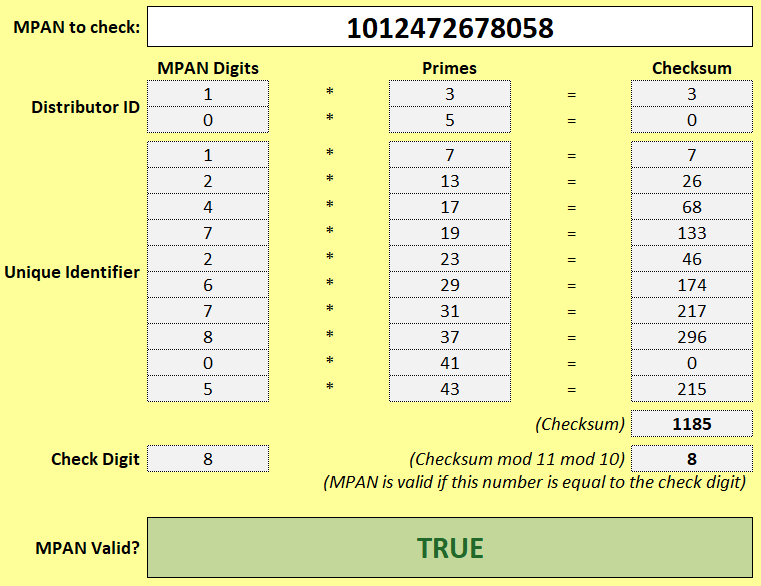
First we calculate the checksum: multiplying each of the first 12 digits by a series of prime numbers, then add them all up:
1 * 3 = 3
0 * 5 = 0
1 * 7 = 7
2 * 13  = 26
4 * 17  = 68
7 * 19  = 133
2 * 23  = 46
6 * 29  = 174
7 * 31  = 217
8 * 37  = 296
0 * 41  = 0
5 * 43  = 215

Checksum = 3 + 0 + 7 + 26 + 68 + 133 + 46 + 174 + 217 + 296 + 0 + 215 = 1185
Then we take the checksum modulo 11, which gives us a number between 0 and 10. (NB 11 was excluded from the series of prime numbers used to calculate the checksum.)
1185 mod 11 = 8
Then we take that number modulo 10, which ensures we are left with a single digit.
8 mod 10 = 8
The last digit of our MPAN is also 8, therefore our MPAN is valid (yay!)
NB this doesn’t prove that the MPAN exists, only that it (probably) has been transcribed correctly. This is just like a credit card number, where you can run an algorithm to check that the card number is valid, but it doesn’t prove that the number has been assigned to an account.
Excel formula to validate MPANs
Here’s the formula, where A1 is the cell containing the MPAN:
=IFERROR(AND(LEN(A1)=13,INT(A1)=A1,MOD(MOD(SUM({3,5,7,13,17,19,23,29,31,37,41,43}*MID(A1,{1,2,3,4,5,6,7,8,9,10,11,12},1)),11),10)=MOD(A1,10)), FALSE)
Let’s break up the formula over several lines, evaluate it step by step, and explain what each part does.
First we check that the MPAN is a 13-digit integer:
=IFERROR(AND(
  LEN(A1)=13,  // check that the MPAN is 13 digits
  INT(A1)=A1, // check that the MPAN is an integer
  MOD(MOD(SUM(
    {3,5,7,13,17,19,23,29,31,37,41,43}*
    MID(A1,{1,2,3,4,5,6,7,8,9,10,11,12},1)
  ),11),10)
  =MOD(A1,10)
),FALSE)
Then we calculate the checksum:
=IFERROR(AND(
  TRUE,
  TRUE,
  MOD(MOD(SUM(
    {3,5,7,13,17,19,23,29,31,37,41,43}*
    MID(A1,{1,2,3,4,5,6,7,8,9,10,11,12},1) // Get the first 12 digits
  ),11),10)
  =MOD(A1,10)
),FALSE)
=IFERROR(AND(
  TRUE,
  TRUE,
  MOD(MOD(SUM( // Calculate the checksum (dot product)
    {3,5,7,13,17,19,23,29,31,37,41,43}*
    {1,0,1,2,4,7,2,6,7,8,0,5}
  ),11),10)
  =MOD(A1,10)
),FALSE)
=IFERROR(AND(
  TRUE,
  TRUE,
  MOD(MOD(SUM( // Calculate the checksum (dot product)
    {3,0,7,26,68,133,46,174,217,296,0,215}
  ),11),10)
  =MOD(A1,10)
),FALSE)
And take the checksum mod 10 mod 11 to get the check digit
=IFERROR(AND(
  TRUE,
  TRUE,
  MOD(MOD(1185,11),10) // Calculate the expected check digit
  =MOD(A1,10) // Get the actual check digit
),FALSE)
=IFERROR(AND(
  TRUE,
  TRUE,
  8
  =8
),FALSE)
And if the expected check digit is the same as the actual check digit, the whole expression will evaluate to TRUE:
=IFERROR(AND(
  TRUE,
  TRUE,
  TRUE
),FALSE)
=IFERROR(TRUE,FALSE)
=TRUE
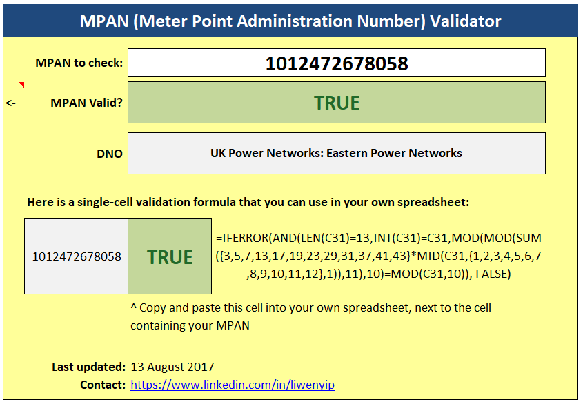
MPAN Validator Spreadsheet
I’ve made a spreadsheet that allows you to validate one MPAN at a time, and includes the single-cell validation formula so you can copy and paste it into your own spreadsheet:
It also shows you how the validation algorithm works:
Get the spreadsheet here.